Passing Images into LLMs
Introduction
Often when I work with LLMs it is with text inputs, but I also use image inputs too sometimes. I continue to spend time learning the internals of the transformer architecture used in decoder style LLMs. But most of my studying has been with text inputs. I was always a little curious, and confused, on how images were passed into LLMs. I just never took the time to dig into it more. Now I am finally getting around to it. This blog post is some notes I'm taking as I learn more about this topic. I write about things so I can better understand them, and my future self is always grateful.
The main motivation for this post was Sebastian Raschka's recent blog post Understanding Multimodal LLMs. I highly recommend reading it. I'm going to focus on learning a subset of the topics that his blog post discusses. I am starting with focusing on what he refers to as Method A: Unified Embedding Decoder Architecture. I may go deeper on other topics in other blog posts, but for now this is a good start for me.
High Level Overview
Large Language Models (LLMs) have revolutionized the way we interact with text, enabling capabilities like natural language generation, reasoning, and conversation. However, their utility isn’t limited to text alone. Modern multimodal models can also understand and process images. How exactly are images passed into these models? That’s what this post aims to clarify.
This post starts with a recap of how transformer-based LLMs process text inputs. We then transition to how images can be converted into sequences of embeddings (just like tokens in text) and fed into LLMs. We’ll look at Vision Transformers (ViT), show how they encode images, and finally explain how these embeddings can be integrated into decoder-style LLMs for multimodal tasks such as image captioning and visual question answering.
Key Takeaways:
- Transformers fundamentally operate on sequences of embeddings—be it text tokens or image patches.
- Images are typically processed by a specialized transformer-based image encoder (like ViT) into a sequence of patch embeddings.
- These image patch embeddings can then be projected into the decoder LLM’s embedding space, allowing the LLM to accept and reason over both text and images.
- Text → tokens → embeddings → transformer
- Images → patches → embeddings → transformer
Recap of Transformer Architecture for Text Inputs
Decoder Style LLMs
We first need to have an understanding of the transformer architecture used in decoder style LLMs. Earlier this year I wrote my first blog post with some notes on the transformer architecture. To get the most out of this post, it would be good to have some familiarity with the transformer architecture. We will give a quick reminder of some basic concepts.
Most LLMs you interact with (like GPT-style models) are decoder-only transformers. In a decoder transformer:
- Input text is first tokenized into discrete tokens.
- Each token is mapped to an embedding vector from a learned embedding lookup table.
- A sequence of token embeddings is passed through the transformer layers (which use self-attention and feed-forward layers).
- The model outputs a hidden state for each token, which is then passed through a classification head to predict the probability distribution over the next token.
We will load one of the SmolLM2 LLM models created by the Hugging Face team. This is not the instruction fine tuned model, but rather the base pre-trained model. This model may not be as well known as some of the other models, but it is a good model to start with since it is really small and easy to run locally.
import torch
import torch.nn.functional as F
from transformers import AutoModelForCausalLM, AutoTokenizer
tokenizer = AutoTokenizer.from_pretrained("HuggingFaceTB/SmolLM2-135M")
model = AutoModelForCausalLM.from_pretrained("HuggingFaceTB/SmolLM2-135M")
model
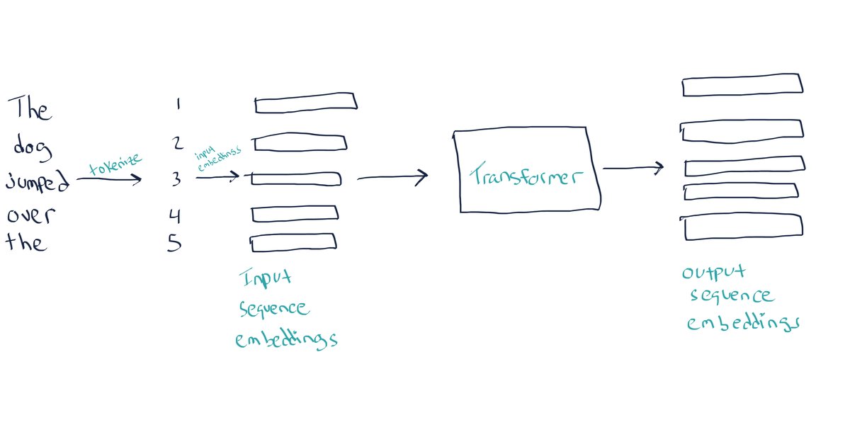
The input to the transformer layers is a sequence of embeddings. In the case of text inputs, the input first gets converted into a sequence of tokens. Then each token is converted into an embedding vector.
Here is the conversion of the input text to tokens ids.
inputs = tokenizer(["The dog jumped over the"], return_tensors="pt")
input_ids = inputs.input_ids
print(inputs)
print(input_ids.shape)
print(input_ids)
Each token id has an associated embedding vector. In the case of this SmolLM2 model, the embedding dimension is 576 and there are 49152 tokens in the vocabulary.
embedding_lkp = model.model.embed_tokens
print(embedding_lkp.weight.shape)
We can get the token embeddings by passing the token ids to the embedding lookup table. Each row of the returned tensor, ignoring the batch dimension, is a vector representation of a token.
embedding_vectors = embedding_lkp(input_ids)
print(embedding_vectors.shape)
print(embedding_vectors)
It is this sequence of embedding vectors that flows through the transformer layers.
The input shape to the transformer layers is (batch_size, sequence_length, embedding_dim)
and the output shape is (batch_size, sequence_length, hidden_size).
You can get the last hidden state by passing the inputs to the model, excluding
the final classification head.
last_hidden_state = model.model(**inputs).last_hidden_state
print(last_hidden_state.shape)
last_hidden_state
Then this final transformer output is passed to the classification head.
The classification head is a single linear layer that maps the hidden state to the logits for the next token.
The output shape of the classification head is (batch_size, sequence_length, vocab_size).
logits = model.lm_head(last_hidden_state)
assert torch.allclose(logits, model(**inputs).logits)
logits.shape
Next we convert the logits to probabilities using the softmax function. While this is useful for visualization and inference, during training we typically use the raw logits directly with CrossEntropyLoss for better numerical stability. Note that we get logits (and after softmax, probabilities) for the next token at each position in the sequence. During inference, we typically only care about the last position's values since that's where we'll generate the next token.
probs = F.softmax(logits, dim=-1)
probs.shape
This next code block shows that at inference time we get the probabilities for the next token at each position in the sequence. It prints the top 5 predictions for each token in the sequence.
K = 5 # Number of top predictions to show
top_probs, top_indices = torch.topk(probs[0], k=K, dim=-1) # Remove batch dim and get top K
# Convert token indices to actual tokens and print predictions for each position
input_text = tokenizer.decode(input_ids[0]) # Original text
print(f"Original text: {input_text}\n")
for pos in range(len(input_ids[0])):
token = tokenizer.decode(input_ids[0][pos])
print(f"After token: '{token}'")
print(f"Top {K} predicted next tokens:")
for prob, idx in zip(top_probs[pos], top_indices[pos]):
predicted_token = tokenizer.decode(idx)
print(f" {predicted_token}: {prob:.3f}")
print()
In summary, the input to the transformer layers is a sequence of embeddings, of shape (batch_size, sequence_length, embedding_dim).
The transformer layers process this sequence and return a new sequence of hidden states, of shape (batch_size, sequence_length, hidden_size).
It is often the case that the hidden size is the same as the embedding dimension, but this is not a requirement. Even if you forget the details of the inner workings of the transformer layers (self attention, etc.), this is a useful mental model to keep in mind. The final classifier layer returns a probability distribution over the next token for each position in the sequence, of shape (batch_size, sequence_length, vocab_size).
Encoder Models
In contrast, encoder-only models like BERT process the entire input sequence at once without causal masking. They often use a special [CLS] token at the start of the sequence, whose final embedding serves as a global representation of the entire input for tasks like classification. Here are some of the key differences between decoder and encoder models:
-
Attention Masking:
- Decoder: Uses causal (or triangular) masked attention to ensure that each position can only attend to previous positions, enforcing an autoregressive quality. This prevents the model from "seeing the future," which is essential for tasks like text generation.
- Encoder: Doesn't require causal masking because it processes the entire input sequence at once. Each token can attend to every other token in the sequence, providing a comprehensive context.
-
Purpose and Data Flow:
- Decoder: Designed for autoregressive tasks, where each output token is generated one by one, conditioning on previously generated tokens. This step-by-step generation is central to tasks like text generation, where each token "builds" upon the preceding tokens.
- Encoder: Designed to encode the entire input sequence into a contextualized representation in one shot, capturing relationships across the whole sequence. It’s typically used in understanding or embedding tasks and classification tasks, where the model needs a holistic view of the input.
Let's load a simple encoder model to illustrate some points.
from transformers import AutoModel
tokenizer = AutoTokenizer.from_pretrained("distilbert-base-uncased")
model = AutoModel.from_pretrained("distilbert-base-uncased")
model
inputs = tokenizer(["The dog jumped over the"], return_tensors="pt")
input_ids = inputs.input_ids
print(input_ids)
print(tokenizer.decode(input_ids[0]))
last_hidden_state = model(**inputs).last_hidden_state
print(last_hidden_state.shape)
In the case of encoder models, the output shape is (batch_size, sequence_length, hidden_size).
In the case of Bert, the hidden size is 768 and a 768 dimensional vector is returned for each token in the input sequence.
When using the encoder output for other tasks, such as classification, we typically take the [CLS] token embedding, which is the embedding for the first token.
last_hidden_state[:, 0, :].shape # `[CLS]` token embedding,
I think it's worth elaborating on the importance of the [CLS] token. Why Use the [CLS] token embedding as the final representation?
When processing text with transformer-based models, each input sequence usually begins with a special token, in this case the [CLS] token. This token doesn’t represent a word or phrase from the input but acts as a placeholder for capturing information about the entire sequence.
During training, the [CLS] token is specifically optimized for sequence-level tasks like classification. For example, in sentiment analysis, the model learns to encode the overall sentiment of the input sequence into the [CLS] token embedding.
As a result, the [CLS] token becomes a rich summary representation of the entire input sequence. Self-attention mechanisms allow the [CLS] token to attend to all other tokens in the sequence. This means it “sees” the entire context of the input. Recall that we typically
don't use the masked attention in the encoder model. Through this process:
- The
[CLS]token learns to aggregate information from all other tokens. - It serves as a global representation, capturing both local token-level features and high-level semantic patterns.
- Adapts dynamically to the task during fine-tuning.
Using the [CLS] token provides a single, fixed-size vector (e.g., 768 dimensions for BERT) that can directly feed into a classifier or other downstream layers.
These concepts are useful to keep in mind when we discuss image encoders later on.
Introducing Images into Transformers and LLMs
Now that we've revisited how transformers handle text inputs, let's explore how images can be incorporated into transformers. Our eventual goal is to understand how to pass images into decoder style LLMs, along side text, to generate text outputs. If you remember that the input to the transformer layers is a sequence of embeddings, then passing in images is no different. We just need to convert the images into a sequence of embeddings suitable for the transformer layers. The fundamental idea: Transformers work on sequences of embeddings. Text tokens are straightforward; they map directly from discrete tokens to embeddings via lookup tables. Images, on the other hand, must be transformed into a sequence of patch embeddings.
Key Insight:
- Text → tokens → embeddings → transformer
- Image → patches → embeddings → transformer
By treating images as a sequence of flattened patches, we can feed them into a transformer architecture—just like we feed tokens into a text transformer.
We’ll first look at how images are handled by Vision Transformers (ViT). Then we’ll explore models like CLIP, which bridge text and image embeddings, and finally see how these image embeddings are integrated into LLMs for multimodal tasks.
Vision Transformers (ViT)
The first architecture we will focus on is transformer-based image encoders. Specifically, we will examine the Vision Transformer (ViT), a model that adapts the transformer architecture from natural language processing to computer vision tasks. The ViT processes images by dividing them into fixed-size patches, embedding these patches as input tokens, and applying a transformer encoder to learn meaningful representations of the input image. Just like the transformer layers process a sequence of token embeddings, the ViT processes a sequence of image patch embeddings, and returns a sequence of hidden states.
Key Steps for ViT:
- Patch Extraction: Divide the image into non-overlapping patches (e.g., 16x16).
- Flatten + Project: Flatten each patch and apply a linear projection to get a 1D embedding vector.
- Positional Embeddings: Add positional embeddings so the model knows each patch’s location.
[CLS]Token: Prepend a learnable[CLS]token to represent the entire image.- Transformer Encoder: Pass this sequence (patch embeddings +
[CLS]) through the encoder layers. - Global Representation: The final hidden state corresponding to the
[CLS]token serves as a global image representation.
The First Vision Transformer
The first Vision Transformer was introduced in the paper AN IMAGE IS WORTH 16X16 WORDS: TRANSFORMERS FOR IMAGE RECOGNITION AT SCALE.

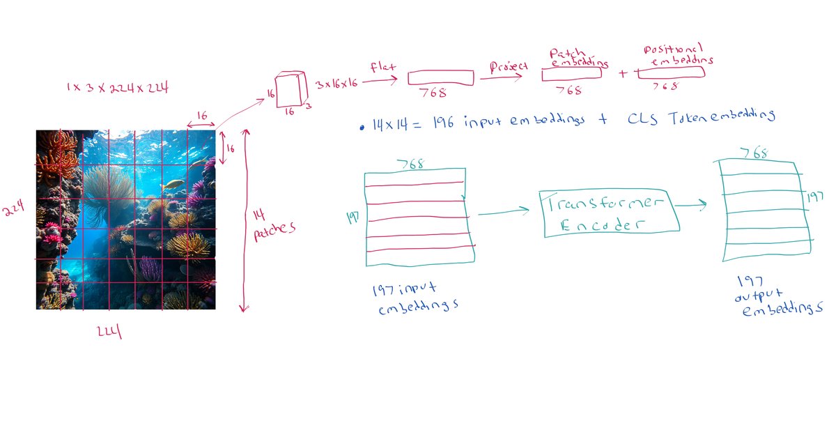
- Split the image into equal sized patches of size 16x16x3 pixels.
- Flatten each patch into a 1D vector of size 16x16x3 = 768.
- Put each flattened patch representation through a linear projection layer to embed each patch into a vector of size 768.
- This is the patch embedding.
- Add a learnable positional embedding to each patch embedding. The positional embeddings help the model understand the spatial relationships between patches
- Also add a
[CLS]token embedding to start of the sequence.
- Pass the sequence of patch embeddings and
[CLS]token embedding, which is a sequence length of 197, through the transformer layers (encoder) to produce a new sequence of hidden states. - The transformed
[CLS]token representation (the first position in the final hidden states) serves as a representation of the entire image and can be used as input to a classifier for downstream tasks.
We can load such a pre-trained ViT model from Hugging Face.
from PIL import Image
image = Image.open("imgs/underwater.jpg")
image
from transformers import ViTImageProcessor, ViTModel
processor = ViTImageProcessor.from_pretrained("google/vit-base-patch16-224-in21k")
model = ViTModel.from_pretrained("google/vit-base-patch16-224-in21k")
model
inputs = processor(images=image, return_tensors="pt")
inputs.keys()
inputs.pixel_values.shape # (batch_size, num_channels, height, width)
# Create patch embeddings from image
patch_embeddings = model.embeddings.patch_embeddings(inputs.pixel_values)
patch_embeddings.shape # [1, 196, 768]
# Get complete input embeddings and pass through encoder manually.
# These embeddings are the patch embeddings plus the positional embeddings.
# As well as the `[CLS]` token embedding.
full_input_embeddings = model.embeddings(inputs.pixel_values)
encoder_outputs = model.encoder(full_input_embeddings)
manual_output = model.layernorm(encoder_outputs.last_hidden_state)
# Get output using full model forward pass
with torch.no_grad():
model_outputs = model(**inputs)
full_model_output = model_outputs.last_hidden_state
# Verify shapes match
assert manual_output.shape == full_model_output.shape
# Verify outputs are identical
assert torch.allclose(manual_output, full_model_output, atol=1e-6)
model_outputs.keys()
model_outputs.last_hidden_state.shape # (batch_size, sequence_length, hidden_size)
model_outputs.last_hidden_state[:, 0, :].shape # `[CLS]` token embedding
In the case of the ViT encoder model, followed by a classification task/head, it is this [CLS] token embedding that we will use as the image representation for downstream tasks. Just like in text encoders, the
[CLS] token in ViT learns to aggregate information from all the image patches through self-attention. During training, this token's representation is optimized to capture the global features needed for image classification. However, it's important to note that this [CLS] token approach is specific to encoder-based vision transformers used for classification tasks. When we later discuss feeding images into decoder style LLMs for tasks like image captioning or visual question-answering, we'll see a different approach where the sequence of patch embeddings themselves are used directly, without needing a [CLS] token.
We've now seen how Vision Transformers process images in a way that's analogous to how text transformers process words. The image is divided into patches (like words in a sentence), each patch is flattened from a 16x16x3 grid of pixels into a 768-dimensional vector, then transformed through a learned linear projection layer to create patch embeddings (like word embeddings). Positional embeddings are added to maintain spatial information (like position encodings in text). The key insight is that both text and image transformers fundamentally operate on sequences of embeddings - the main difference is just in how we create these embeddings from the raw input. For ViT, it's through patch extraction, flattening, and linear projection; for text, it's through token lookup tables.
CLIP
CLIP (Contrastive Language-Image Pre-training) represents a significant milestone in connecting visual and textual understanding. Unlike the original ViT which focused solely on image classification, CLIP learns to understand the relationship between images and their natural language descriptions. CLIP was created by OpenAI.
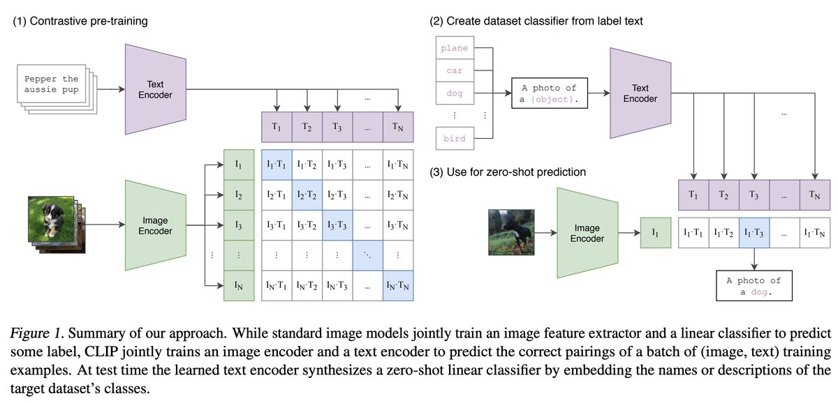
CLIP's architecture consists of two encoders working in parallel:
A text encoder (transformer) that:
- Processes sequences of text tokens
- Produces a final representation using the
[CLS]token - Projects this representation into a normalized embedding space
An image encoder (can be ViT or other CNN architecture but let's focus on ViT) that:
- Processes images as sequences of patch embeddings
- Transforms these through transformer layers
- Uses the
[CLS]token for final representation - Projects into the same normalized embedding space (Note: While CLIP can also use ResNet CNN architectures that don't use patches, we're focusing on the ViT version)
The key innovation is the contrastive learning process:
- Pairs of images and text descriptions are encoded into the same embedding space
- The model learns to maximize similarity between matching pairs while minimizing similarity for non-matching pairs
- This creates a shared semantic space where similar concepts in either modality (image or text) end up close together
This aligned semantic space enables powerful capabilities:
- Comparing images and text directly
- Finding semantic similarities across modalities
from PIL import Image
from transformers import CLIPModel, CLIPProcessor
model = CLIPModel.from_pretrained("openai/clip-vit-large-patch14")
processor = CLIPProcessor.from_pretrained("openai/clip-vit-large-patch14")
image = Image.open("imgs/tropical_island.jpg")
image
model
inputs = processor(text=["a photo of an island", "a photo of a plane"], images=image, return_tensors="pt", padding=True)
outputs = model(**inputs)
logits_per_image = outputs.logits_per_image # this is the image-text similarity score
print(logits_per_image)
probs = logits_per_image.softmax(dim=1) # we can take the softmax to get the label probabilities
probs
The image was compared to the two different text descriptions and the model was able to correctly identify that the image was more similar to the text description of an island. We can get the embeddings separately as well:
inputs
inputs.keys()
print(processor.decode(inputs.input_ids[0]))
print(processor.decode(inputs.input_ids[1]))
inputs.pixel_values.shape
# Get embeddings separately
image_features = model.get_image_features(inputs["pixel_values"])
text_features = model.get_text_features(input_ids=inputs["input_ids"], attention_mask=inputs["attention_mask"])
print(f"Image embedding shape: {image_features.shape}")
print(f"Text embeddings shape: {text_features.shape}")
temperature = 1 # I think there is a temperature parameter to be set here.
logits = (image_features @ text_features.T) / temperature
logits
Since we have loaded a version of CLIP with the ViT image encoder, we can also get the final transformer hidden states, corresponding to each of the input image patches.
- Input image size is 224x224 pixels
- Using patch size of 14x14 pixels
- 16x16 grid = 256 patches
- Add
[CLS]token at the start to get a 257 sequence length
The embedding dimension is 1024.
# Get vision model outputs with hidden states
vision_outputs = model.vision_model(inputs["pixel_values"], output_hidden_states=True)
# Get final hidden states (sequence of patch embeddings_
final_patch_embeddings = vision_outputs.last_hidden_state # Shape: [batch_size, num_patches + 1, hidden_size]
final_patch_embeddings.shape
outputs = model.vision_model(inputs["pixel_values"], output_hidden_states=True)
outputs.keys()
outputs.last_hidden_state.shape
These are the transformed input patch embeddings plus the [CLS] token output embedding.
In summary, CLIP uses a dual-encoder architecture with both a vision encoder and a text encoder. When using the ViT-based image encoder, an image is processed into 256 patch embeddings plus a [CLS] token embedding (total 257 tokens with dimension 1024 for ViT-large). CLIP can be used in two distinct ways: First, for image-text comparison, where the [CLS] tokens from both encoders are projected into a shared space and compared using cosine similarity (scaled by temperature). Second, the sequence of 256 patch embeddings (excluding [CLS]) can be extracted from the vision encoder and passed to decoder-style LLMs, enabling the LLM to process detailed visual information alongside text. This second approach forms the foundation for many multimodal LLMs, which we'll explore later.
SigLIP: an improved version of CLIP
SigLIP (Sigmoid Loss for Language Image Pre-Training) represents an evolution of the CLIP architecture, maintaining the same dual-encoder structure but introducing key improvements in how similarity is computed between image and text embeddings. While CLIP uses a softmax-based approach that compares each image against all text descriptions in a batch, SigLIP adopts a sigmoid-based similarity measure that evaluates each image-text pair independently. This change, along with its corresponding loss function modifications, leads to more robust training and better performance on downstream tasks. Despite these improvements, the fundamental way we interact with the model remains similar to CLIP - we can still use it for image-text comparisons or extract visual features for use with decoder LLMs (more on this later). There is a great notebook here.
from transformers import AutoModel, AutoProcessor
model = AutoModel.from_pretrained("google/siglip-so400m-patch14-384")
processor = AutoProcessor.from_pretrained("google/siglip-so400m-patch14-384")
image = Image.open("imgs/sci_fi_ship.jpg")
image
model
texts = ["an alien ship", "sc-fi ship in the forest", "sci-fi ship"]
# important: we pass padding="max_length" as that's how the model was trained
inputs = processor(text=texts, images=image, padding="max_length", return_tensors="pt")
for k, v in inputs.items():
print(k, v.shape)
with torch.no_grad():
outputs = model(**inputs)
logits_per_image = outputs.logits_per_image
confidence_scores = torch.sigmoid(logits_per_image) # Independent confidence scores
print(f"{confidence_scores[0][0]:.1%} confidence score for '{texts[0]}'")
print(f"{confidence_scores[0][1]:.1%} confidence score for '{texts[1]}'")
print(f"{confidence_scores[0][2]:.1%} confidence score for '{texts[2]}'")
Note the main difference between SigLIP and CLIP is how the similarity scores are computed
-
CLIP uses softmax:
- Outputs are normalized across all text candidates
- Scores sum to 1
- Each score represents a relative probability compared to other options
-
SigLIP uses sigmoid:
- Each score is independent
- Scores are between 0 and 1 but don't sum to 1
- Each score represents a confidence measure for that specific pairing
We can also just use the image encoder to get the final transformed patch embeddings:
# Get vision model outputs with hidden states
vision_outputs = model.vision_model(inputs["pixel_values"], output_hidden_states=True)
# Get final hidden states (sequence of patch embeddings)
final_patch_embeddings = vision_outputs.last_hidden_state # Shape: [batch_size, num_patches + 1, hidden_size]
final_patch_embeddings.shape
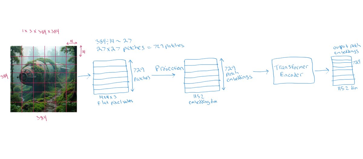
SigLiP takes as input the 384x384 image and the patch size is 14x14 pixels. This leads to 27*27=729 patch embeddings.
Question to self: Does it not use the [CLS] token?
vision_outputs.keys()
vision_outputs.pooler_output.shape
Question to self: Maybe the the pooler_output is the pooled representation of the final patch embeddings?
Vision Language Models
Finally, we can discuss one way in which images can be passed into decoder style LLMs along with text. Remember I was motivated to learn more about this by Sebastian Raschka's recent blog post Understanding Multimodal LLMs. In that blog post, one of the approaches for passing images into decoder style LLMs is referred to as "Method A: Unified Embedding Decoder Architecture approach". This is the approach I want to discuss a little bit more here. Why? Because this was my main motivation for learning more about the topic of multimodal LLMs. I knew how text was tokenized and passed into decoder style LLMs, but I didn't know how images were handled.
Now that we have learned about transformer image encoders i.e Vision Transformers (ViTs), we already know how images are processed and encoded as sequences of patch embeddings. And we saw how those patches are first projected into the input patch embedding space of the image encoder, and then fed into the transformer layers. The output of the image encoder is a sequence of patch embeddings. Let's look at a diagram of the role of the image encoder one more time:
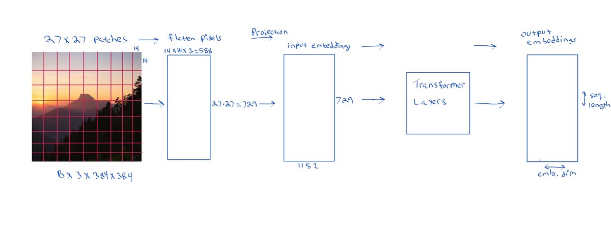
Now suppose we have a decoder style LLM that we want to use for a multimodal task. We would like to feed in an image along with text. For example we could feed in an image along with a question about the image such as "What is in the image?" or "What is the image about?". The recipe for how to do this is as follows:
- Encode the image using a pre-trained ViT image encoder, such as CLIP or SigLIP etc., and get the sequence of transformed patch embeddings as output by the image encoder.
- Then project the resulting output embeddings into the input token embedding space of the decoder LLM
- This is done to ensure the image embeddings are in the same embedding space as the text embeddings for the decoder LLM. This is the role of the multimodal projector/adapter in the diagram below.
- Concatenate the projected image patch embeddings with the text token embeddings
- Feed the concatenated sequence into the decoder style LLM
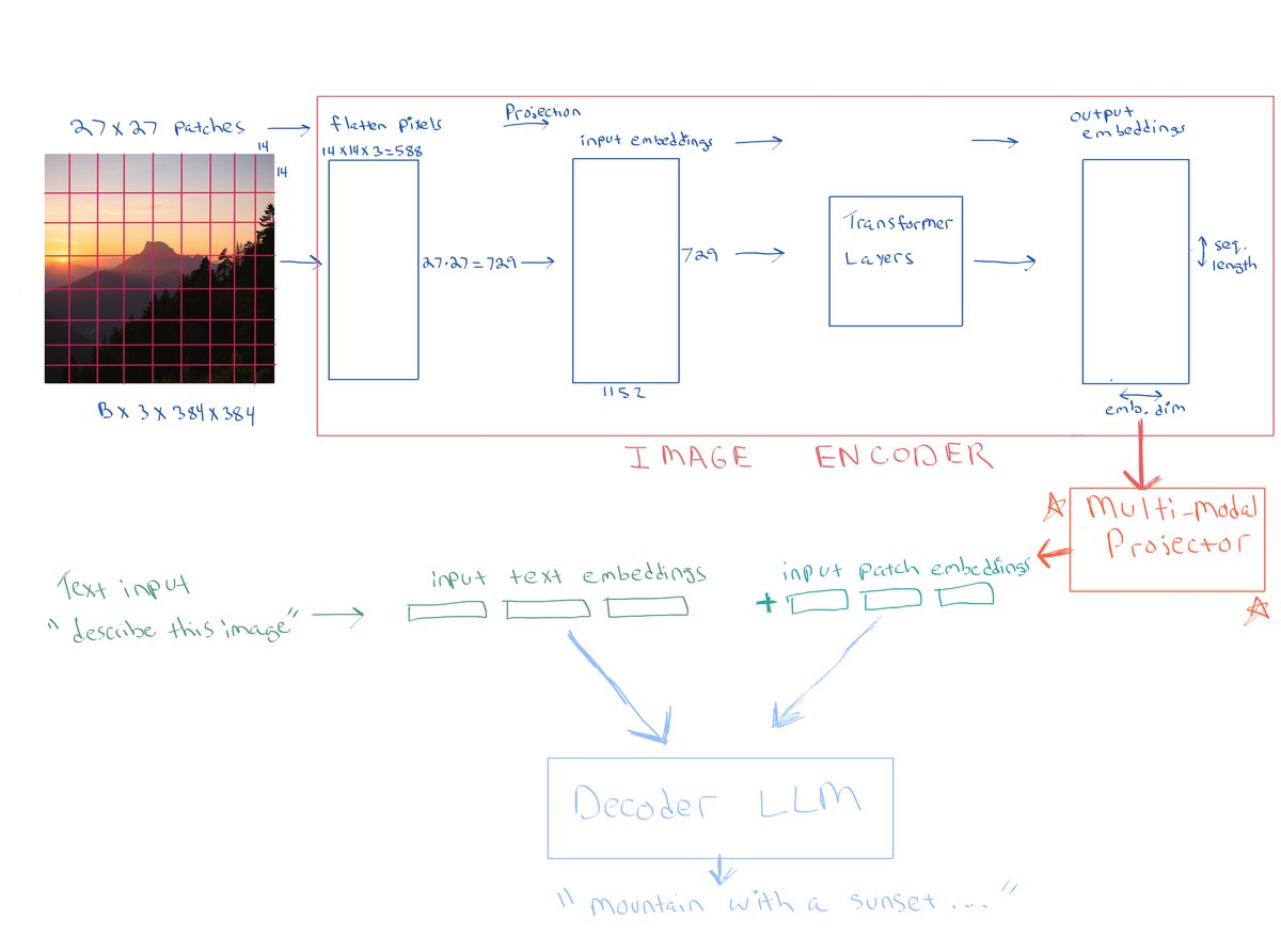
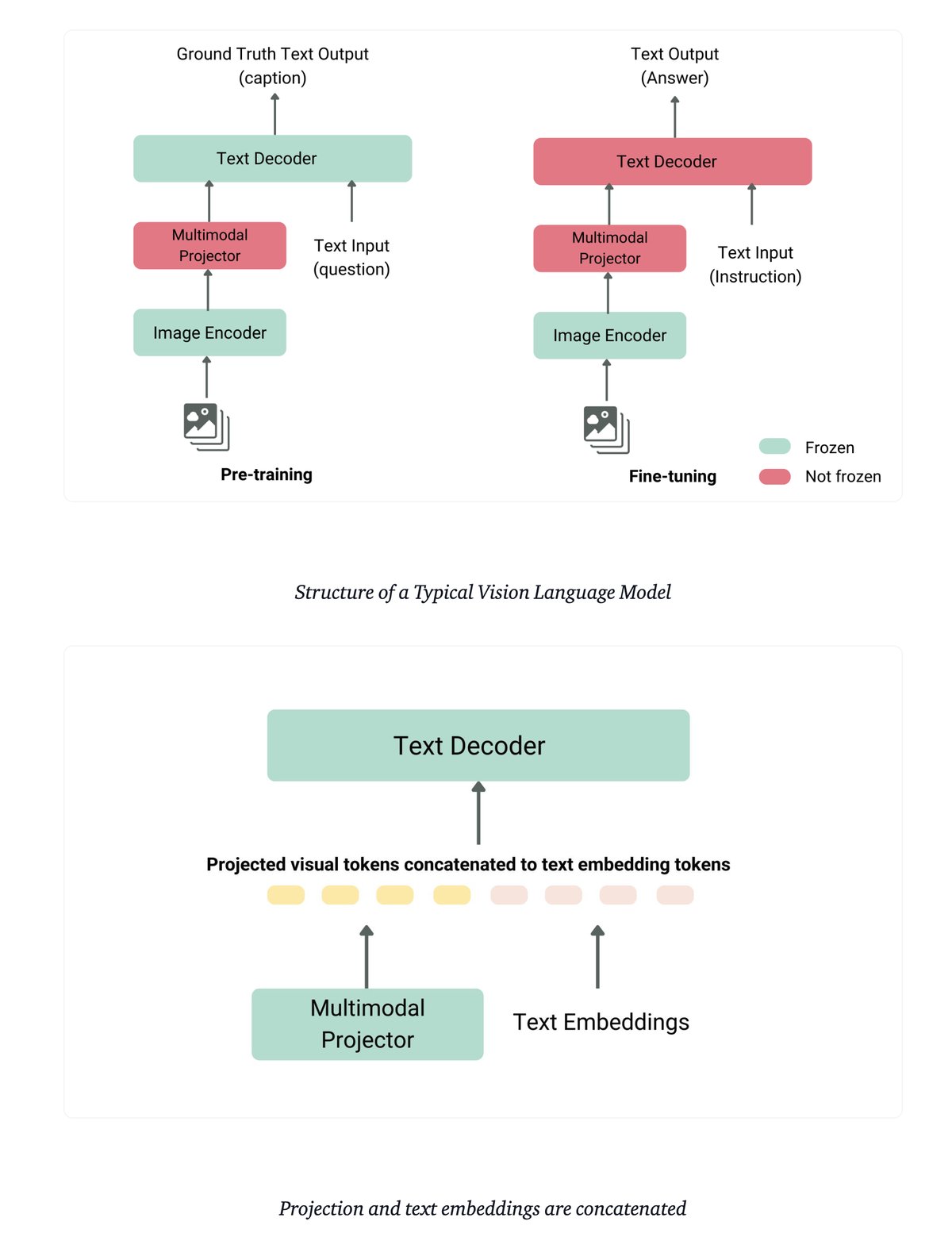
There are many different ways to train a vision language model. I will describe one common approach related to the setup above. In the first stage of training, the pre-trained image encoder is frozen along with the decoder LLM. The part that is trained in this first stage is the multimodal projector/adapter(often a dense neural network). The dataset needs to consist of image-text pairs, for example image and caption pairs. The multimodal projector is designed to align image and text features by inputting images and generated questions into the model and evaluating its outputs against the corresponding ground truth captions. In the second stage of training, the decoder LLM is unfrozen and trained together with the multimodal projector. Again, this is one such approach for training a vision language model.
There is an excellent explanation in this blog post from Hugging Face Vision Language Models Explained . I have borrowed this diagram from that blog post which also illustrates this common approach of training a vision language model.
Conclusion
I’ll admit, I’ve run out of steam here, and I’ve only scratched the surface. There’s a great deal more to learn. The resources listed below offer plenty of reading and exploration opportunities. As I continue to revisit these topics and dive deeper into new research, I hope to gain a better understanding of the ever-expanding world of multimodal models. Personally I would like to go deeper into fine-tuning small decoder style LLMs for multimodal tasks.
Resources (in no particular order)
Multimodal LLMs
AI Visions Live | Merve Noyan | Open-source Multimodality
Vision Language Models Explained
LLaVA: Large Language and Vision Assistant - website
Visual Instruction Tuning - paper
Improved Baselines with Visual Instruction Tuning - paper
PaliGemma – Google's Cutting-Edge Open Vision Language Model
PaliGemma: A versatile 3B VLM for transfer: Paper
PaliGemma 2: Announced when I finished writing this post
Gemma explained: PaliGemma architecture: Google for Developers Awesome-Multimodal-Large-Language-Models
SmolVLM - small yet mighty Vision Language Model
Vision Transformer (ViT)
AN IMAGE IS WORTH 16X16 WORDS: TRANSFORMERS FOR IMAGE RECOGNITION AT SCALE
Vision Transformer (ViT) - Hugging Face Documentation
Training CLIP Model from Scratch for an Image Retrieval App
Vision Transformer (ViT: Hugging Face)
Fine-Tune ViT for Image Classification with 🤗 Transformers